This vignette presents a technical description of the daedalus model in its current state. It should be noted daedalus is in constant development; we will attempt to keep this document as updated as possible during the lifespan of the model. If you encounter any issues, contact the package developers or raise a GitHub issue.
Rationale
The daedalus package is the implementation of a deterministic epidemiological and economic model of the emergence and spread of respiratory pathogen pandemics in countries. Specifically, daedalus tracks
Health impact in terms of infections, hospitalisations, deaths and years of life lost (YLL), and
-
Economic impact in terms of GDP losses from:
- Economic sector closures and workforce depletion due to infection, hospitalisation or death
- Present and life-time economic losses from missed education
- Human life losses using the value of statistical life approach
Presently, we have equipped daedalus with parameters to simulate seven potential pathogens (influenza A 2009, influenza A 1957, influenza A 1918, SARS-CoV-1, SARS-CoV-2 pre-Alpha variant, SARS-CoV-2 Delta and SARS-CoV-2 Omicron BA.1, see this table on pathogen parameters) across 67 countries. In addition, daedalus allows the user the flexibility to incorporate additional respiratory pathogen and/or country parameters and data, as considered appropriate for their use case.
The following sections present a technical description of the epidemiological and economic components of daedalus. For examples of its implementation in research case studies, see
The original description of daedalus and application to the UK during the COVID-19 pandemic in Haw et al. (2022)
Study of the societal value of SARS-CoV-2 booster vaccination in Indonesia in Johnson et al. (2023)
Study of promoting healthy populations as a pandemic preparedness strategy in Mexico in Johnson et al. (2024)
Epidemiological model
Model structure
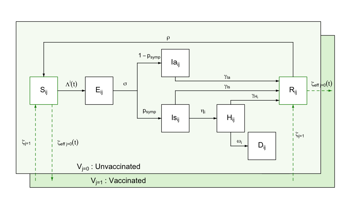
daedalus simulates a country’s population split into seven possible disease state compartments. Model compartments are stratified by age-sector sector \(i\) and vaccination \(j\) classes.
A susceptible individual \(S\) can become exposed to the virus and enter a latent state \(E\), from which they can develop either a symptomatic \(I_s\) or asymptomatic \(I_a\) infection. Whereas asymptomatic infected individuals are assumed to always recover, symptomatic ones can either recover \(R\) or develop a more severe condition requiring hospitalisation that would lead to either recovery \(H_r\) or death \(H_d\). We assume different lengths of hospital stay for this compartments, after which individuals transition to the recovered \(R\) or death \(D\) compartments.
Ordinary differential equations
\[ \begin{aligned} & \frac{dS_{i,j}}{dt} = \zeta_{eff_{j=0}}(t) S_{i,j=0}(t) - \Lambda_{i,j} (t) S_{i,j}(t) + \rho R_{i,j}(t) - \zeta_{j=1} S_{i,j=1}(t)\\ & \frac{dE_{i,j}}{dt} = \Lambda_{i,j} (t) S_{i,j}(t) - \sigma E_{i,j}(t) \\ & \frac{dIa_{i,j}}{dt} = (1 - p_\text{symp}) \sigma E_{i,j}(t) - \gamma_{I_a} I_{a_{i,j}}(t) \\ & \frac{dIs_{i,j}}{dt} = p_\text{symp} \sigma E_{i,j}(t) - \gamma_{I_s} I_{s_{i,j}}(t) - \eta^i I_{s_{i,j}}(t) \\ & \frac{dHr_{i,j}}{dt} = \eta^i (1 - \text{HFR}_{i}) I_{s_{i,j}}(t) - \gamma_{H_r} H_{r_{i,j}}(t) \\ & \frac{dHd_{i,j}}{dt} = \eta^i \text{HFR}_{i} I_{s_{i,j}}(t) - \gamma_{H_d} H_{d_{i,j}}(t) \\ & \frac{dR_{i,j}}{dt} = \zeta_{eff_{j=0}}(t) R_{i,j=0}(t) + \gamma_{I_s} I_{s_{i,j}}(t) + \gamma_{Ia} Ia_{i,j}(t) + \gamma_{Hr} Hr_{i,j}(t) - \rho R_{i,j}(t) - \zeta_{j=1} R_{i,j=1}(t)\\ & \frac{dD_{i,j}}{dt} = \gamma_{Hd} Hd_{i,j}(t)\\ \end{aligned} \]
Should be noted that whilst some model parameters vary over time (e.g., \(\zeta_{eff_{j=0}}(t)\) effective vaccination rate scaled for available susceptible population) others are assumed fixed (e.g., \(\sigma\) constant rate of \(E \rightarrow I\) progression), which is indicated by \((t)\).
One parameter that varies endogenously is the age-specific mortality rate \(\omega^i\); mortality rates for all groups increased by 160% when the total number of individuals in the ‘hospitalised’ compartment exceeds the country-specific surge hospital capacity available for responding to the outbreak.
Note that, as default, daedalus ships a
collection of pre-defined parameter sets that represent historical
respiratory pandemic pathogens (see this table
on pathogen parameters), as contained in daedalus.data.
These can be saved as an object of class daedalus_infection
and modified by the user to be then passed to the model function
[daedalus::daedalus()].
Age-sector classes
There are 49 age-sector classes \(i\) in daedalus: four age \(i \in 1:4\) groups \(([0, 5), [5, 20), [20-65), 65+)\) and, given population in \(i=3\) (20–64 years old) represents unemployed adults ofr working age, 45 economic groups \(i \in 5:49\) (see in the section on the economic model below).
Vaccination classes
As a default, daedalus further disaggregates the population into the vaccination classes \(j \in 1:2\) of unvaccinated and vaccinated. We assume only the population in the susceptible and recovered compartments can be vaccinated, given transition rate \(\zeta_{\text{eff}_{j=0}}(t)\), which is determined by the user (see this table on vaccination scenario parameters). Vaccinated individuals can lose their immunity and transition back to an unvaccinated class, given rate \(\rho\).
Model transition parameters
daedalus can simulate nine different pathogens (influenza A 2009, influenza A 1957, influenza A 1918, SARS-CoV-1, SARS-CoV-2 pre-Alpha variant, SARS-CoV-2 Delta and SARS-CoV-2 Omicron BA.1) with pathogen-specific transition (see this table on pathogen parameters).
| Parameter | Definition |
|---|---|
| \(\Lambda_{i,j} (t)\) | Force of infection by age-sector and vaccination class |
| \(\sigma\) | Rate of progression from exposed to infectious |
| \(p_\text{symp}\) | Proportion of exposed individuals becoming symptomatic |
| \(\eta^i\) | Probability of hospitalisation by age, conditional on symptomatic infection |
| \(\gamma_{Ia}\) | Recovery rate for asymptomatic infections |
| \(\gamma_{Is}\) | Recovery rate for symptomatic infections |
| \(\gamma_{Hr}\) | Recovery rate for hospitalised individuals |
| \(\gamma_{Hd}\) | Death rate for hospitalised individuals |
| \(\rho\) | Rate of waning immunity (recovered to susceptible) |
| \(\zeta_{eff_{j=0}}(t)\) | Vaccination rate |
| \(\zeta_{j=1}\) | Vaccine protection waning rate |
Table: Definition of model transition parameters.
Seed and force of infection
For any given pathogen, we assume a seed of \(10^{-7}\) infections, all of which are further assumed to be symptomatic.
The force of infection \(\lambda_{i,j} (t)\) accounts for the infection contributions of symptomatically \(I_{s_{ij}}(t)\) and asymptomatically \(I_{a_{ij}}(t)\) infected individuals in the community and in workplaces.
We let \(\delta I_{\text{comm}}^i(t)\) and \(\delta I_{\text{work}}^i(t)\) denote the number of infected individuals in the community and the workplace, respectively, weighted by their infectivity given
\[ \begin{aligned} & \delta I_{\text{comm}_{ij}}(t) = v_{eff_{j=1}} (I_{a_{i \in 1:4,j}}(t) \epsilon + I_{s_{i \in 1:4,j}}(t))\\ & \delta I_{\text{work}_{ij}}(t) = v_{eff_{j=1}} (I_{a_{i \in 5:49,j}}(t) \epsilon + I_{s_{i \in 5:49,j}}(t)) \end{aligned} \]
where \(\epsilon\) is the relative infectiousness of an asymptomatically infected individual relative to a symptomatic one, and \(v_{\text{eff}_{j=1}}\) the reduced susceptibility of a vaccinated individual relative to an unvaccinated one of the same age.
The force of infection from the community \(\lambda_{\text{comm}_{i,j}} (t)\) on a susceptible individual is thus modelled as
\[ \lambda_{\text{comm}_{i,j}} (t) = \beta (t) \cdot \sum_{i'} m_{i,i'} \sum_{j'} \delta I_{{\text{comm}}_{i',j'}} (t) \]
where \(\beta(t)\) represents a time-varying contact rate scaling factor, determined by social distancing interventions simulated, and \(m_{i,i'}\) is the (symmetric) person-to-person contact rate between age group \(i\) and \(i'\).
The force of infection within the workplace \(\lambda_{work_{i,j}} (t)\) is modelled as
\[ \lambda_{\text{work}_{i,j}} (t) = \beta (t) \cdot \Phi_i(t) \cdot \sum_{i'=0}^{i'=N} C_{i,i'} \sum_{j'} \delta I_{\text{work}_{i',j'}} (t) \]
where \(C_{i,i'}\) is a contact matrix specific to the workplace, and \(\Phi_i(t)\) is a scaling factor determined by economic closure interventions simulated.
Lastly, the force of infection from infected individuals in the community to susceptible workers \(\lambda_{\text{comm}\rightarrow\text{workers}_{i,j}} (t)\) (i.e., infected individuals from the community attending shops) is given by
\[ \lambda_{\text{comm}\rightarrow\text{workers}_{i,j}} (t) = \beta (t) \cdot \Phi_i(t) \cdot \sum_{i'=0}^{i'=N} {C \rightarrow W}_{i,i'} \sum_{j'} \delta I_{{\text{comm}}_{i',j'}} (t) \]
where \(C \rightarrow W_{i,i'}\) is a contact matrix specific to consumers attending workplaces.
The total force of infection acting on susceptible individuals is then assumed to be an addition of the above. For conciseness, this can be taken as
\[ \Lambda_{ij} (t) = \lambda_{\text{comm}_{ij}} (t) + \lambda_{\text{work}_{ij}} (t) + \lambda_{\text{comm}\rightarrow\text{workers}_{i,j}} (t) \]
however, it should be noted that the force of infection within the workplace \(\lambda_{work_{ij}} (t)\) is a column vector of length 45, given the number of economic sector classes in the model, whilst \(\lambda_{\text{comm}_{ij}} (t)\) and \(\lambda_{\text{comm}\rightarrow\text{workers}_{i,j}} (t)\) are of length 49, encompassing all age-sector classes.
Disease transition rates
| Parameter | Symbol | Influenza 2009 | Influenza 1957 | Influenza 1918 | Covid Omicron | Covid Delta | Covid Wild-type |
|---|---|---|---|---|---|---|---|
| Basic reproduction number | \(R_0\) | 1.58 | 1.80 | 2.50 | 5.94 | 5.08 | 2.87 |
| Probability symptomatic | \(p_{\text{sympt}}\) | 0.669 | 0.669 | 0.669 | 0.592 | 0.595 | 0.595 |
| Relative infectiousness (asymptomatic:symptomatic) | \(\epsilon\) | 0.58 | 0.58 | 0.58 | 0.58 | 0.58 | 0.58 |
| Latent period (days) | \(1/\sigma\) | 1.1 | 1.1 | 1.1 | 4 | 4 | 4.6 |
| Infectious period asymptomatic (days) | \(1/\gamma_{Ia}\) | 2.5 | 2.5 | 2.5 | 2.1 | 2.1 | 2.1 |
| Infectious period symptomatic (days) | \(1/\gamma_{Is}\) | 2.5 | 2.5 | 2.5 | 4 | 4 | 4 |
| Infection-induced immune period (days) | \(1/\rho\) | 365 | 365 | 365 | 365 | 365 | 365 |
| Length of hospital stay leading to recovery (days) | \(1/\gamma_{Hr}\) | 5 | 5 | 5 | 5.5 | 7.6 | 12 |
| Length of hospital stay leading to death (days) | \(1/\gamma_{Hd}\) | 5 | 5 | 5 | 5.5 | 7.6 | 12 |
| Age specific parameters* | |||||||
| Hospitalisation rate given symptomatic infection (\(\text{days}^{-1}\)) | \(1/\eta^i\) | ||||||
| 0-4 years | 358.7 | 1851.9 | 13.7 | 73006.1 | 80405.4 | 148750.0 | |
| 5-19 years | 359.5 | 158.7 | 15.6 | 133.7 | 25.4 | 47 | |
| 20-64 years | 912.4 | 1851.9 | 50.4 | 5900.4 | 4638.8 | 8581.7 | |
| 65+ years | 161.7 | 9.3 | 6.6 | 35.8 | 8.1 | 15 | |
| Hospital fatality ratio conditional on symptomatic infection leading to hospitalisation (%) | \(\text{HFR}^i\) | ||||||
| 0-4 years | 25.3 | 13.5 | 8 | 1.0 | 1.0 | 1.0 | |
| 5-19 years | 16.0 | 13.5 | 8 | 14.9 | 12.4 | 12.4 | |
| 20-64 years | 24.2 | 13.5 | 8 | 5.2 | 5.3 | 5.3 | |
| 65+ years | 1.6 | 13.5 | 8 | 3.2 | 3.5 | 3.5 |
Table: Pathogen parameters. A different
pathogen profile can be created by the user by generating a list object
specifying these parameter values (see list structure for these
pathogens in daedalus.data::infection_data). *Note disease
severity progression is modelled with competing rates (e.g., for
individuals in the \(I_a\) compartment,
of recovery \(\gamma_{I_s}\) vs
hospitalisation by age \(\eta^i\));
where NA values are specified, we assume these individuals cannot
undergo the respective disease severity transition.
Vaccination
Vaccination is implemented as a series of default pre-determined vaccine investment scenarios, which can be modified as necessary by the user.
| Advance vaccine investment | Start time (days) | Rate (% per day) | Uptake limit (%) | Efficacy* (%) | Waning period (mean, days) |
|---|---|---|---|---|---|
| None | 365 | 0.14 | 40 | 50 | 270 |
| Low | 300 | 0.29 | 50 | 50 | 270 |
| Medium | 200 | 0.43 | 60 | 50 | 270 |
| High | 100 | 0.5 | 80 | 50 | 270 |
Table: Vaccination parameters. These pre-specified
parameters can be modified by the user and/or additional strategies can
be added by generating a list object with the same structure (see
daedalus.data::vaccination_scenario_data). *Note the
default version of daedalus only models vaccine efficacy
against infection; for use cases with added functionality to simulate
efficacy against other clinical severity end-points see Johnson et al. (2023).
Modelling economic losses
daedalus assigns monetary values to three key types of model outcomes that we interpret as losses: the years of life lost due to epidemic-related deaths, economic activity lost due to worker illness and epidemic mitigation measures, and years of education lost due to worker illnesses and epidemic mitigation measures.
The life-years lost and education-days lost valuations models are explained in more detail in their own vignettes (see links below), and here we focus on the valuation of economic losses.
Value of life-years lost: Calculated using a value of a statistical life approach based on the country-specific gross national income (as the broadest possible data source); see this vignette on how the value of life-years lost is calculated.
Value of education-days lost: Calculated using an approach based on the present value of future earnings; see this vignette on how the value of educational time lost is calculated.
Economic activity losses
We calculate the cost of economic closures by each of 45 \(k\) sectors in terms of lost gross value added (GVA). daedalus runs in continuous time, with outputs calculated at daily time steps.
The daily GDP generated by a country in the absence of closures is composed of the maximum daily GVA \(y_k(t)\) for each sector \(k\). There is a 1:1 mapping of the 45 economic sectors and the age-sector population strata \(i \in 5:49\). For conciseness, in this section we index economic sectors and age-sector classes only as \(k\).
Formally, the maximum possible GDP generated \(Y_0(t)\) by all economic sectors \(m_S\) in the absence of mandated closures (i.e., as a result of non-pharmaceutical interventions that restrict economic workplace capacity) at time \(t\) is defined by
\[ Y_0(t)=\sum_{k=1}^{m_S}y_k(t), \]
where all economic sectors contribute their daily GVA \(y_k(t)\).
If an economic sector is, however, affected by closures on a given day, we estimate its GVA losses as
\[ y_k(t) = y_k(0) \cdot (1 - \kappa_k(t)) \]
where \(y_k(0)\) is the respective sector’s daily GVA in the absence of closure and \(\kappa_k(t)\) its relative openness (i.e., from 0 to 1, where 0 is completely open and 1 completely closed). We thus assume sectors contribute $0 USD in GVA on day \(t\) if completely closed.
In addition to GVA losses from closures, economic sectors can lose productivity whilst being open given depletion of their workforce (i.e., due to self-isolation, sickness, hospitalisation or death). \(x_{k}(t)\) is the proportion of the workforce contributing to economic production in sector \(k\) out of the total workforce \(N_k\) on day \(t\). As the workforce of a sector is depleted, we assume a smaller fraction \(\hat{x}_{j}(t)\) will be available to contribute to production given
\[ \hat{x}_{k}(t) = x_{k}(t) \left(1 - \sum_{j=0}^{1} \left( \frac{I_a^{j,k}(t) + I_s^{j,k}(t) + H^{j,k}(t) + D^{j,k}(t)}{N_k} \right) \right). \]
The total GDP generated at time \(t\) is then
\[ Y(t) = \sum_{k=1}^{m_S} y_k(t) \hat{x}_{k}(t), \]
and the GDP loss compared to the maximum is
\[ \int_{t=0}^t \left( Y_0(t) - Y(t) \right)dt. \]