Under-reporting and Age Structure

Why the age distribution is informative

In the motivating setting for vrcmort, the observed VR data show a sharp pattern after conflict starts:

• trauma deaths increase (as expected),
• non-trauma deaths decrease (implausibly), and
• the age distribution of non-trauma deaths shifts younger.

If you believe the underlying non-trauma mortality burden among older adults has not collapsed overnight, this is strong evidence that registration completeness has become age-selective.

This vignette explains how vrcmort uses age structure to model under-reporting.

An illustration

The plot below is a stylised illustration of the pattern the model is designed to capture.

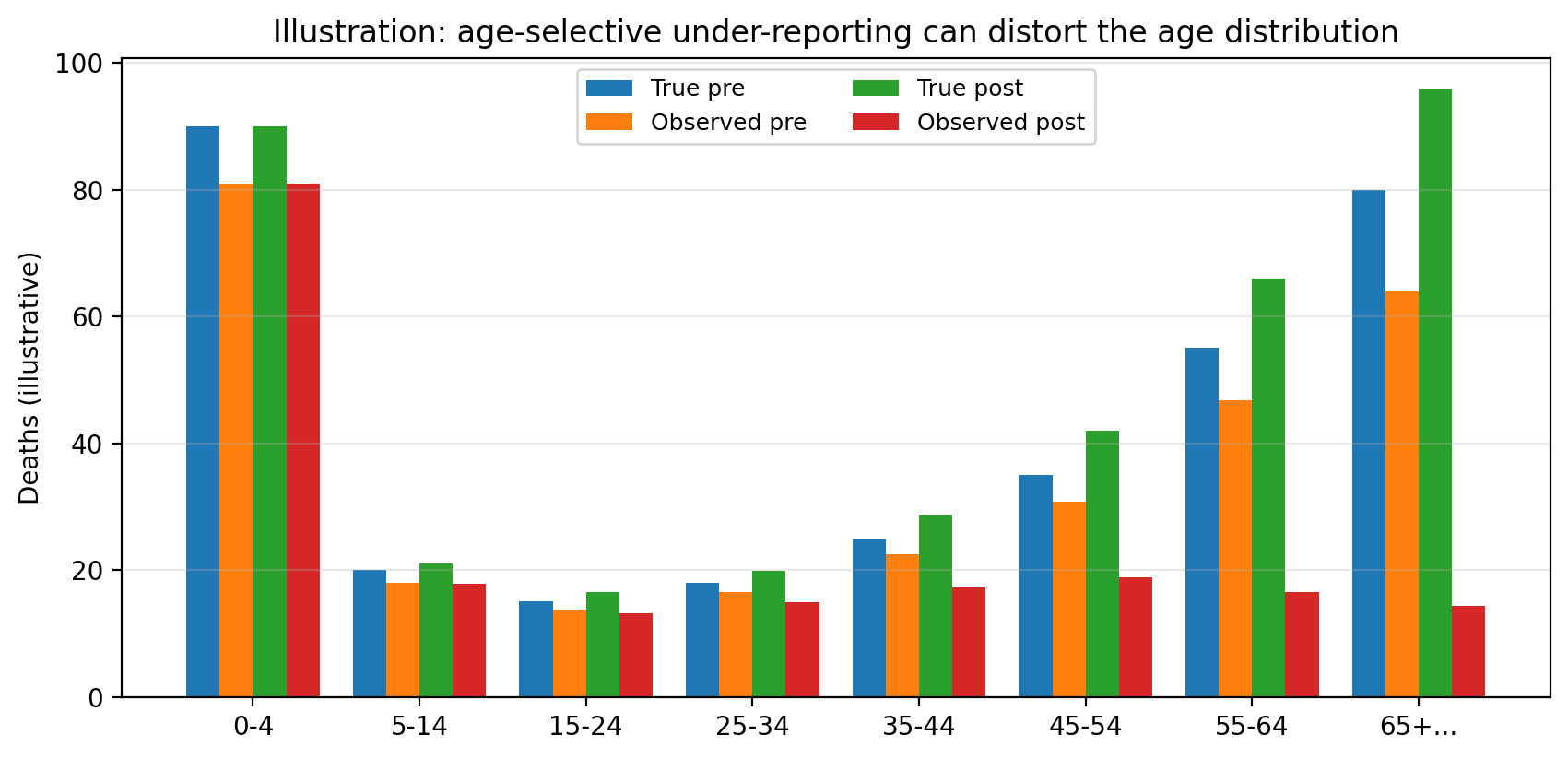
Pre-conflict, observed deaths roughly track true deaths in all age groups. Post-conflict, observed deaths fall steeply in older ages even if the true age profile remains similar.

What vrcmort does in the base model

In the base model, reporting completeness is modelled on the logit scale:

$$\text{logit}(\rho_{r,t,a,s,g}) = \kappa_{0,g} + \kappa_{post,g} \cdot \text{post}_t + \ldots + \text{agepen}(a,g,t).$$

The age penalty is designed to be:

• non-negative,
• monotone non-decreasing with age, and
• only active after conflict begins.

A conceptual form is:

$$\text{agepen}(a,g,t) = -\delta_a \cdot \mathbb{1}[g=\text{non-trauma}] \cdot \text{post}_t,$$

with $\delta_a \ge 0$ and $\delta_a$ increasing with age group.

Why monotone?

Monotonicity encodes a weak structural belief: if the system collapses in a way that removes older deaths, it is unlikely to remove age 65+ deaths while still reliably recording age 45-54 deaths.

It also stabilises inference by preventing the model from fitting a highly wiggly age pattern in completeness.

How the monotone penalty is implemented

In Stan, monotonicity is implemented via positive increments between successive age groups:

$$\delta_1 = 0, \quad \delta_{a+1} = \delta_a + \Delta_a, \quad \Delta_a \ge 0.$$

The increments $\Delta_a$ have priors that control how steep the penalty can become.

Practical data preparation advice

Choose age groups with a clear interpretation

Use age groups that reflect both epidemiology and data density.

A common starting point is 5-year or 10-year bins up to a final open-ended group (for example 65+).

If older ages are very sparse even pre-conflict, consider coarser bins at older ages.

Avoid changing age group definitions across time

If you redefine age groups over time, the model will interpret changes in the age distribution as a change in mortality or completeness.

Keep the denominator consistent

Because the expected count depends on exposure

$$\mu = E \cdot \lambda \cdot \rho,$$

large errors in the age-specific exposure can mimic reporting collapse.

If you have displacement flows, try to apply them to the age-sex population structure so that the exposure reflects the people actually at risk in each region-month.

Diagnosing age-selective under-reporting in data

vrc_diagnose_reporting() provides basic summaries, but for age-specific work you will often want a focused plot.

Here is a template (pseudo-code) for plotting age distributions by period and cause.

library(dplyr)
library(ggplot2)

vr_long %>%
  mutate(period = if_else(time < t0, "pre", "post")) %>%
  group_by(period, age, cause) %>%
  summarise(y = sum(y, na.rm = TRUE), .groups = "drop") %>%
  group_by(period, cause) %>%
  mutate(frac = y / sum(y)) %>%
  ggplot(aes(x = age, y = frac, group = period)) +
  geom_line() +
  facet_wrap(~ cause) +
  labs(y = "Share of recorded deaths")

The key pattern to look for is a post-conflict shift of non-trauma deaths towards younger ages.

Inspecting inferred completeness by age

After fitting, you can extract the inferred completeness surface and aggregate it by age.

fit <- vrcm(
  mortality = vrc_mortality(~ 1),
  reporting = vrc_reporting(~ 1),
  data = vr_long,
  t0 = t0,
  chains = 4,
  iter = 1000
)

rho <- posterior_reporting(fit)

# Summarise completeness by age and period
rho %>%
  mutate(period = if_else(time < t0, "pre", "post")) %>%
  group_by(period, cause, age) %>%
  summarise(rho_mean = mean(rho_mean), .groups = "drop")

If the model is behaving as intended, you should see a larger post-conflict drop in inferred completeness for older ages in the non-trauma cause group.

Limitations and extensions

Age structure is informative, but it is not magic.

• If conflict truly changes the age distribution of non-trauma deaths (for example because older adults leave the region, or because access to care changes differentially by age), you need population and covariates to reflect that.
• If there is systematic misclassification (for example non-trauma deaths being coded as trauma, or as ill-defined), a misclassification extension may be needed.

The current base model is designed as a starting point that you can stress test and extend.